
Deep Learning has become a hammer of sorts that can nail down almost any ML problem. While deep learning is undoubtedly solving many problems that most other ML algorithms cannot, it has also made many people who are just starting out in the field and many who have been in the field for a long time believe that it can be used to solve any problem as long as you stack up enough layers and neurons. This naivety has been particularly heightened by easily available frameworks like Keras and TensorFlow, cheap computational power in the form of Amazon AWS and GCP, and a very open and supportive ML community. At present, anyone can easily take a few online courses, read a few papers and write code for a state-of-the-art CNN to recognize Handwritten digits, and call themselves an ML engineer. Even I am guilty of doing the same, and I have done so with very little money and a laptop worth less than $500. And it is because of this that people have forgotten the two most important parts of Machine Learning: Math and Data.

Machine Learning is, after all, Data Driven AI, and your model will be only as good or as bad as the data you have. You can’t have a dataset of car images and expect to use it to classify cats and dogs (unless you use transfer learning), and in the same way, you cannot use linear regression to train a model on a dataset that does not have linear correlation. In this article, I’ll be talking about data, data correlation, and how your choice of an ML algorithm should not be depend on how state-of-the-art an algorithm is, but rather on how your data is.
So how important is data?
Energy Disaggregation is the use of Machine Learning to figure out the kind of electrical devices you might have in your home using features like meter data, weather, locality etc. When I was working on a project to do the same, my Neural Network could never predict the electrical devices properly. No matter how wide or deep a network I made, I could hardly get an accuracy above 55%. It took me a long time to realize that it wasn’t a problem with my model, but rather a problem with my data.
To do this project, I was using a dataset that I got off of some website. The data was neither properly labeled, nor was it good, as there were some very erratic power values that did not correspond to the weather data at the same time. All this meant that no matter how good my model was, it could have never done its job properly as the data itself was really bad!
But then what is good data?
It’s very hard to answer a question like that. I now tend to not use data that is not from a verifiable source. A verifiable source could be Kaggle, KDNuggets, a company’s or a country’s open source datasets, and datasets that researchers have used to solve whatever problem you are solving. Sometimes getting the right data to do a project can be the hardest part of doing that project, especially if you are trying to do something new. Most of the projects that I have done in machine learning (Electrical Engineering related), I had to get from PhD scholars and researchers. So point to keep in mind: Do not hesitate to ask experts for data!
Once you have procured your data, even if it is from a verifiable source, you still need to check if it is good or not. This is when data wrangling and data visualization will come in use. Numpy, Pandas and Matplotlib are great for data wrangling and visualization. By visualizing data, you can figure out, not only the kind of data correlation you have (more on that later), but also how your data looks, the different features of the data, and if the features correspond with the output.
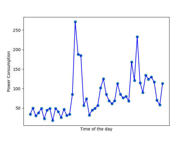
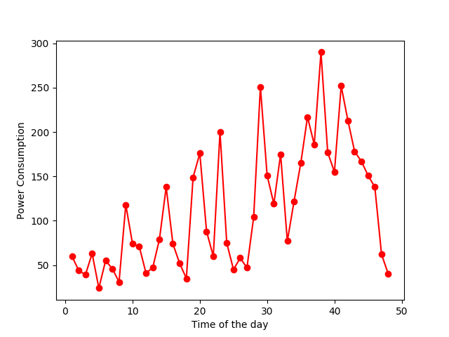
For example, the two images below show power usages of homes throughout the day. It doesn’t take machine learning to figure out that the erratic curve in image 2 is noisy or irregular data (something that I have dealt with a lot in electrical engineering). On the other hand, the rise and fall of the curve in the first image can be attributed to the increase in power usage in the mornings and evenings, and less power usage in the night. If I were training a model to predict power usages, I’d use the first data. Data visualization helps you understand if the data you are using will help your purpose or not.
Coming to Data Correlation
Early in this post, I mentioned that you cannot use linear regression to model a nonlinear dataset. The opposite is also true, if you have a linearly correlated dataset, even the best CNN will give you a poorer result than a simple model like linear regression. Data correlation is the way in which one set of data may relate mutually with another set. In terms of machine learning, it can be thought of as how your features correspond with your output.
For example, in this dataset of brain size versus body size, you can see that the brain size is almost directly proportional to the body size, that is, as the body size increases, so does the brain size. This is what would be called a linear correlation as the data follows a straight line (there is a more formal definition of linear correlation, but that will do for now).
Not all data is linearly correlated, for example, this curve of ice cream sales versus temperature has an inverted U shaped graph. It could mean that once the temperature rises above a certain value, people might not want to leave their homes and go to ice cream shops. So using something like Linear Regression does not make sense on this dataset.

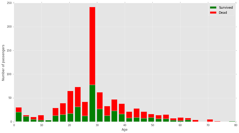
However, it becomes very hard to figure out how your data may be correlated if you have more than two features. In this case, you can use data visualization again to figure out how individual features may correlate with the output. In the Kaggle Titanic competition, there are a lot of features and you can also make many features by combining the features that are already present. You can separately see the correlation of sex with survival, and age with survival. From these visualizations it becomes very obvious how sex and age played a very big role in deciding who might have survived aboard the Titanic. Visualizations can also help you filter out useless features: there is no correlation between embarked port and survival.

Getting to the Math
Visualisation might help a lot, but if you are someone who’d rather see numbers and stats, then there are a lot of ways to find out how data is correlated. Pearson’s Correlation Coefficient helps you find out the relationship between two quantities. It gives you the measure of the strength of association between two variables. The value of Pearson’s Correlation Coefficient can be between -1 to +1, where 1 means that they are highly correlated, 0 means no correlation and -1 means that there is a negative correlation (think of it as inversely proportional).
T-Test is also another correlation coefficient used to determine whether there is some correlation between two values. Other popular correlation coefficients include the Spearman rank order correlation and Pearson’s Rank Correlation. All these coefficients have their own advantages and drawbacks and you should know when to use which one.
An important thing to note here though is that if you have a large dataset and if you get a small coefficient, say 0.4, then it’s not necessarily bad. It could mean that there is a large statistically significant correlation in your data. Another important thing to note is that correlation may not mean causation, and just because two variables are related, does not mean that one directly caused the other. The people aboard the Titanic did not die just because they were male and aged 28. It’s just that a large number of them died because officers were saving “Women and Children First”.
The importance of data correlation comes into play when you have a dataset with many features. One may be tempted to think that a larger number of features will help our model make better predictions. But that is incorrect. If you try to train a model on a set of features with no or very little correlation, you will get highly inaccurate results. Age of the person who wrote a particular digit in MNIST could be another feature, but it really wouldn’t help us make better predictions. When dealing with high dimensionality datasets, it is important to filter out these non-correlated features and use a lesser number of highly correlated features to train a model.
Datasets with more features or higher dimensions is a recent problem as data collection and storing has never been easier. More often than not, many datasets have features with similar information, which acts as noise in the system and increases complexity. Some features also have very little variance. If your output has a lot of variance, then do you think a feature with a constant value (low variance) will significantly improve your model? NO! To figure out the importance of each feature in a dataset, rank correlation is used.
Rank correlation techniques help us find out which features have more correlation with the output as compared to other features. One of the most popular rank correlation methods in Machine Learning is the Principal Component Analysis. It uses principal components to find out which low dimensionality set of features from a high dimensional dataset can correctly capture the most meaning from a dataset. With fewer dimensions, data visualisation also becomes easier. Random Forests and Decision Trees are also extremely powerful tools that can be used to find data correlation. They work by finding out the statistical usages of each feature, making it easier to figure out what the most important features are.
And finally,
How can you use all that you have learned to figure out which algorithm to use?
Data correlation and data visualisation is important because with them, you can get an intuition of which Machine Learning algorithm might work best on a given data set.
Take a look at the brain vs body size data again. Do you think using deep learning or neural networks would make sense? Obviously not! While both a neural network and linear regression will be able to fit this data, linear regression is far less computationally expensive will train faster than a neural network.
In case your data does not have a linear correlation, you could consider using polynomial regression, SVM’s or Random Forests. On large datasets however, these might be more computationally expensive to train than a small neural network.
When working on Image Recognition problems, it’s always better to use Convolutional Neural Networks. On the other hand, NLP and time series problems are better modelled by Recurrent Neural Networks and LSTMs (Long Short Term Memory).
Another factor that you should take into account while choosing an algorithm to use is whether you are doing regression or classification. Neural networks are really good at classification tasks. On the other hand, while neural networks can be better at doing classification, they aren’t always the best at regression. While you could perform a lot of data augmentation and fine tune a lot of parameters, a fairly simple SVM might perform better.
That’s all Folks!
Sources:
The brain size vs body size image was taken from Siraj Raval’s tutorial on implementing linear regression from scratch.
The Titanic Graphs were sourced from Ahmed Besbes blog on how to score 0.8134 in Kaggle Titanic Challenge.
Other diagram were taken from an article on data correlation from mathsisfun.com
