A Hacker’s Guide to Understanding Controllers

Hey! In this article, I’ll be talking about controllers: What they are, what are their types and why we use them. Controllers are one of the most important, but often, the most neglected part of a system design and even I didn’t know much about them until I had to use them in a project I was working on very recently. While I was researching into controllers, I did not come across any good material on them and most of what was online was written in terms of what might be asked during an exam, but not in terms of designing and making your own project. So this article will be more of a hacker’s guide of sorts to understand controllers and implementing them in projects.

I was recently building a robot that would take a position as input and it would then move to that position. This was a simple project in which the robot could move only in one direction, that is, forwards and backwards and it would calculate its distance from a wall and that would be it’s position. It was supposed to be an easy project that shouldn’t have taken more than a few hours to complete, but even after three days, my robot would still not stop at the position given to it as input. There would always be an error of a few centimeters. It took me a long time to realize that what I was missing was a feedback loop and an error corrector in my system. Both these problems are solved by a very simple device(or code, which we’ll talk about later) called a controller.

Controllers are very important, but neglected at the same time. They are used in systems to change and maintain a system state. In my case, it was to change the position accurately and maintain it. Pretty much any electrical, mechanical, robotic, embedded…any system really, has a controller in them. Motors use controllers to to maintain speed, quad copters use them to maintain height or to stay level, cars use them to move and robots use them to pick up objects and perform tasks. Controllers are so versatile, that despite being decades old, we still haven’t found an alternative for them(partly because we don’t need to).

So what is a controller?

Formally, a controller can be a digital/analog circuit or a software, that tries to keep a variable like temperature, speed, position or angle set at a certain value called the set point or the set value. A controller does this by having a feedback loop that looks at an error signal(which is the difference between the real signal and the desired signal). The job of the controller is to minimize that error signal. If a motor is spinning too fast, reducing the error will reduce the speed, if the temperature is too low, it will increase the temperature etc.

It is very important to have that feedback loop as that is what will tell the controller whether it is at the desired set value or not. Once it reaches the set value, the controller will try to keep the system at the set value.

We use controllers because it helps keep our system stable. Stability means that the system will stay at the set point. If the motor on a crane wasn’t stable(at the same speed), then a crane operator would never be able to pick up or move any object. Stability in a system is important and a controller helps us maintain that. You also want your system to be robust and disturbance resistant. If your robot moves from a carpeted floor to a slippery marble floor then the friction changes, but you still want your robot to perform similarly. This ability to perform the same task under different conditions, environments or disturbances makes the system robust.

Another thing that we might want to look at while designing a system is optimality: Is the system performing at its optimal state? If a robot is moving from point A to point B, is it taking the shortest path? This is an optimality problem and controllers can be designed to take that into account.

As you can see, controllers are very robust and versatile objects. Now that we have pretty much understood what a controller is, and why we might want to use one, let’s start designing our own controller.

Note: The following sections are a bit math intensive, but it shouldn’t be a problem if you know your basic maths really well. I have tried my best to explain everything I do, but in case you do find anything that I have not explained well enough or if I have made some mistake, do mention it in the comments.

Designing the simplest controller

When I was first trying to design a position robot, it was always a few centimeters off from the set value or my desired position. What I did at that time was design what is probably the world’s simplest controller, which looked kind of like this:

Let’s say that our desired position is = y

Let’s say our current position is = x

So our error is = e = y-x

What this means is that if e is positive, then our car still hasn’t reached the set value or has probably stopped before it has reached the set value. If e is negative, then it has overshot the set value and we need to make the car move backwards.

Let the speed of the car be = U

So what if we design a controller like this:

What this system of equations means is that if our error is greater than 0, or our robot has not reached the desired point yet, then we set the robot’s speed to U_max. This will make the robot move towards the desired position. In case the robot has a negative error, we will have to move it backwards and so we set its speed to -U_max. And, if the error is 0, then the robot has already reached it’s position and it does not have to move. Seems reasonable right? I mean, intuitively, that is what we want our robot to do. Or is it?

A system like this will give an output as shown above. Here the value on the y-axis represents the error and the x-axis the time. The reason for such an output is simple: At first, the speed of the car increases and we accelerate until we hit zero error. But, the speed of our robot is still pretty high, it’s still at U_max, so we overshoot and now the error becomes negative. At this point, our controller switches the speed to -U_max and eventually we start going backwards, gaining speed and we overshoot again. And this gets repeated over and over.

This kind of control is known as Bang-Bang Control. When we switch between two extremes, the controller reacts harshly to even small errors and causes the kind of output we see.

So what were the problems in this system?

Well, for one, our response to the error signal e was constant. But this should not be the case. Instead the closer we are to the set value or the smaller our error signal is, our response needs to get smaller and smaller, until it is zero when we get to the set point.

Another thing you might have noticed was that our response, U, was jerky or unstable. It would randomly change values that would cause the response to change rapidly over time.

None of these are characteristics that we want a controller to have. A controller should not only be robust and stable, but it should also have a very smooth response. In short, we want our response to be large when the error signal is large and we want the response to decrease with a decrease in the error signal, that is, we want the response to be proportional(or inversely proportional) to the error signal.

The Proportional Controller

In the previous problem we saw that the response was same irrespective of the error signal. However, we want a controller that has an output that is proportional to the error. To model that, we use a proportional controller. The formula of a proportional controller looks something like this:

where e is the error signal, and k_p is called the proportionality gain.

In this case, a small error will yield a smaller value of U, and a large error will yield a larger value of U. Also, in the case where e is negative, the value of U will also be negative. So we get a nice and smooth response unlike our Bang-Bang controller in the previous example.

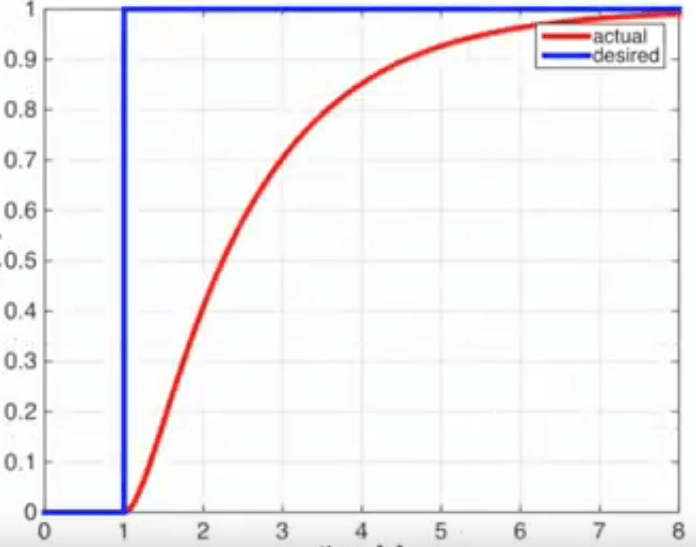
Say we want our robot to move 60 mm or 6 cm. So we make our set point as 6 cm and we run the program. We get an output like this.

Amazing right! We got a smooth response and the system is stable. Well, not really. If you check the graph properly, you’ll see that our position is actually 5.8 and not 6. This is because once our error signal decreases up to a certain level, the value of k_pe becomes very less. This means that the value of U becomes very less and no changes occur. This error is more or less constant and is known as the steady state error. So what if we increase the value of k_p? We could do that, but that would cause our value to overshoot again. So, even though the system will have a smooth response, it will not achieve tracking, or it will not be able to reach the correct value of set point.

The proportionality gain tends to act like a spring, by increasing the value, the system tends to overshoot. But the advantage of the proportional controller is that for a large error, it gives a very fast response and this will come in handy when we will design more complex systems.

But for now, we need a system that can further reduce the error and get the real value closer to the desired value.

The Integral Controller

If you look at the graph of the proportional controller, it actually did a good job at reducing the error quickly in the beginning, but then, it lost steam and was not able to reduce the error any further. And for a large value of K_p, our controller overshoots.

While we are using the value of error to define our response, what we are not taking into account is the amount of error buildup over time(marked in red). By trying to reduce this buildup of error over time, we should be able to get our error down to zero as this error will also include the steady state error of we got from the P controller.

An Integral can be used to calculate this error buildup over time. The I Controller looks something like this:

That might look like a confusing equation so we’ll break it down into parts. The first part is U which is our systems response. This is followed by K_i which is our Integral Gain constant. That is followed by the integral symbol. We integrate form 0, the starting time to t, our ending time. e(t) is our error signal as a function of time, which is a fancy way of saying that it represents our error at any given time. What the integration part means is that we sum up all the error values from 0 to t and then we multiply it with our Integral Constant.

The I controller on its own has a very slow response. This is because it needs the error to build up before it can start working. So an I controller on its own will act like a damped system. We can overcome this however by using the fast responsiveness characteristic of the P controller. Hence we define a PI or a Proportional-Integral Controller as:

All I did was add the equation of the P and I controller to get the above equation. The PI controller takes into account both the effects of the proportion of error and the integral of the error over time. By changing the values of K_p and K_i, we can change the amount of proportional and integral response we want our system to have. I’ll talk about how to choose the values of K_p and K_i later. But for now, its safe to know that our system will be able to reduce all errors and maintain stability. In fact, PI controllers are so good at their job that more than half of the controllers used today are PI controllers. Everything from the cruise control in your car to the speed regulators in your fan uses a PI controller.

However, we still haven’t solved one problem: The problem of a smooth response. A PI controller does have a smooth response, and it is smooth enough for most systems, but for many sensitive systems, you might need a slower response time. For example, to design a system that mixes chemicals in specific amounts, you might want to mix the chemicals slowly and you definitely do not want the quantities to overshoot their desired values. To do this, we add a derivative term in our system.

The Derivative Controller

The derivative of our error gives the slope of the error signal at that time. The slope represents the rate of change of our error at that time. The derivative controller looks like this:

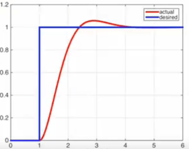
K_d is the derivative gain and it acts as a damper that makes sure that our system response is slow and that it never overshoots the set value. By combining P and D controllers, we get a PD controller:

These controllers are widely used in aerial robotic applications. By choosing appropriate values of K_p and K_d, we can get a stable system that does not overshoot. Some points to consider for PD controllers are:

1)If we choose a small value for K_d, the system might overshoot like so

2)If we increase the value of K_p too much, we will have a system with a fast response, but we will also have oscillations in the system like so

3)If however, we have a system with a large value of K_d, then we will have an over damped system like so

Enter PID controllers

We now know what P, PI and PD controllers are. To have a system where you can take advantage of the different properties of P, I and D, we use a PID controller. By choosing smaller or larger values of the constants, we can give the system more or less properties of different controllers.

There are essentially, 3 parts to that equation that you can tweak while designing a system. They are the Proportional Gain or K_p, the Integral Gain K_i and the Derivative Gain K_d. Tweaking these different values have the following effects:

K_p: It has a Fast Response, it improves Stability, But there is a constant Steady State Error and there is no tracking. A small value of K_p increases stability, but causes a large steady state error. A larger value tends to make the system overshoot.

K_i: Improves tracking, but it has a very slow rate of response and may cause oscillations. It also increases the disturbance rejection of the system.

K_d: By increasing the derivative gain, we tend to make the system overdamped. The derivative is also sensitive to noise as the slope at a time will change if you have a noisy signal.

OK, So now that we know what a controller is, what the different parameters are and how tweaking each parameter can cause a different output, we can now finally move on to learning how to implement controllers. But before that, I should probably answer the next question first.

What’s the difference between a Controller and a Micro-controller?

Many people don’t know the answer to this, and after searching online for the better part of a day, even I could not find any material online that properly answers this question, so I’ll try my best to answer it.

A controller and a micro-controller are actually quite different from each other. A micro-controller is a device that can be used to control a system. It has I/O ports that can take both digital and analog inputs and outputs and based on some input signals, it does some calculations and gives an output signal. While a micro-controller is a hardware device, a controller, is a mathematical process or function that can be used to get a desired result. This means that a PID controller can be implemented inside a micro-controller and most of the time, that is what is done today. For example, in my example robot project, I had a distance sensor that could measure the position of my robot, this would be given as feedback to my micro-controller that would then calculate the error and the value of response and tell the wheels of my robot to move based on that.

How to Implement a Controller

We’ll be implementing a controller using a micro-controller. We’ll be implementing a motor speed controlling system. To do so, we’ll need to first tell the micro-controller what speed to maintain. We also need a feedback loop that tells the micro-controller what speed the motor is running at currently. To change the speed of the motor we usually control the voltage using a converter.

Using these two values we can calculate the error value. This error value will then need to be fed into the equation for whatever controller you want to use. By tweaking the values of K_p, K_i and K_d, we can make sure that when we change the speed of the motor, there are reduced oscillations and that the system is stable. The value outputted by the controller can be then given into the voltage converter which will in turn change the speed of the motor.

Sources:

Many of the images in this tutorial were taken from online courses on Coursera and edX. The courses were “Aerial Robotics” by Prof. Vijay Kumar from the University of Pennsylvania and “Control of Mobile Robots” by Dr. Magnus Egerstedt from Georgia Institute of Technology. They are both amazing courses and are highly recommended.